A STUDY OF A SIMPLE 1 DIMENSIONAL STACKED SYSTEM COLLAPSING using a physics game engine1
This is a documentation of the results obtained from playing around with a physics engine. A game physics engine. How useful could that be? If it's accurate for the application, how bad can it be? How is accuracy determined?
Questions, questions, questions. Too tiresome, let me skip to the answers and then go back and revisit the questions.
- A body cannot be simultaneously both rigid and deformable
- A rigid body, obeying d'Alembert's principle, forces energy dissipation of crushing to occur in the lower block
- A non-rigid upper block passes diminished jolt amplitude to the 'roofline' but does so by dissipating energy internally, through deformation and failure
- A discrete model, even highly idealized, is a dynamic problem with more than one degree of freedom if upper is not rigid
- The simplest representation, which conforms to typical discrete inelastic models, has TWO aggregate, generalized coordinates
- A 1D solid slab and spring model with many members, and which fails, has a propensity for crush-up whether or not crush down occurs
Surprised? Not me. But maybe you disagree. I'll be back to disclaim, explain and support these notions, along with showing some results, as time permits. In the meantime, either yawn or rip me a new one, either one is fine.
The topic is not specific to the mechanics of any particular collapse.
EXAMPLE
Typical cusp example, hopefully much is self-explanatory.
- constant mass
- varying strength
- true 1D in 3D
- dynamics calculated using spheres
- rendered as slabs with height = diameter of spheres
- camera tracks with topmost member
- sequence ends at arrest
That covers most of what isn't obvious.

A comparison of displacement for two stretch values, 0.2 and 0.05, everything else the same. The collapses go to completion, being a mix of crush up and down until the top is completely crushed. Blue is the larger stretch value.

Nearly identical through the mixed phase, but the phase lasts longer for the smaller stretch, and this sets the difference between them until the end is reached, where once again the crush down (only) phase lasts longer since there's further to go.
This example also illustrates the characteristic appearance that these particular simulations produce when there is mixed crush direction. A little almost-parabola riding atop a larger almost-parabola.
CASE 1- MIXED CRUSH
Jumping into this without disclaimers is ill-advised. Nothing here is meant to represent a real structure, let alone any particular building. The simulator has not finished basic validation against knowns, nor has the energy consumed in breaking connections been fully profiled over the range of conditions of these examples. I'm using unit masses! Even if flawless, the inherent limitations of a discrete 1D analysis limit the application. There is some hope it will be illuminating, regardless.
The first case to examine closely is one in which a mix of crush up and down occur simultaneously in the beginning, but crush-up stops before the topmost connection is broken. Crush down goes to completion, but the final connection at the top does not break at the end.
The case of the top connection surviving has been encountered frequently. The reason is simple, and it goes to why my earlier simulations shown in the Crush Down Models thread were able to shatter the lower 90% without suffering damage. An upper block of only two slabs has a single slab bearing down on the connection, versus many slabs bearing down. If the lower block (Zone A) is being crushed down simultaneously, what takes place at the top is a low gravity crush up; that is, dynamics of the upper block (Zone C) is simply the solution of a crush up scenario in an accelerated frame wrt ground, i.e., a falling elevator. Zone C can rarely survive this pummeling even in the accelerated frame but, if any part of it can, it's the topmost part.
Back to the case at hand. First, an animation of the early drop, which ends at the point we see the topmost connection survive. Again, the camera tracks with the top, centered on a point below. This has proven to be the most useful view to capture the motion, though it might take a little time to feel comfortable. Each slab starts with two connections, shared above and below, except for the top and bottom slabs of Zones A and C. The number of remaining connections (2, 1, 0) to a given slab is reflected in the color of the slab.

The ratio of crush up/down is seen directly in the color bands. To achieve this particular mix, the entire upper block Zone C was set to the same connection strength throughout, to a value which is slightly higher than that of the top connection of the lower block Zone A. Later, this run will be compared to a model differing only by a very slight increase in the connection strength of Zone C, to make more of the upper block survive the initial drop.
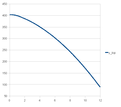
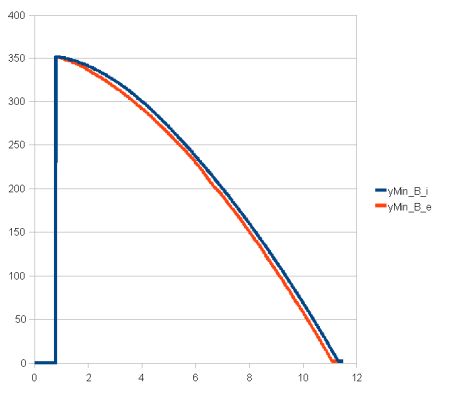
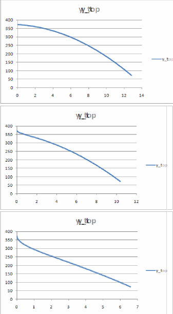
Next, some graphs to get an idea of the dynamics for this simulation. Position of the very top over time:
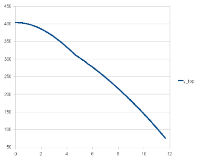
Once again, the superimposed pair of curves are seen, corresponding to an initial phase of mixed crush direction followed by a crush down only phase. A kink is visible in the curve where crush up ceases, leaving the top two 'intact' slabs riding down on Zone B, the crush layer. The jolt can be seen in the velocity curve:
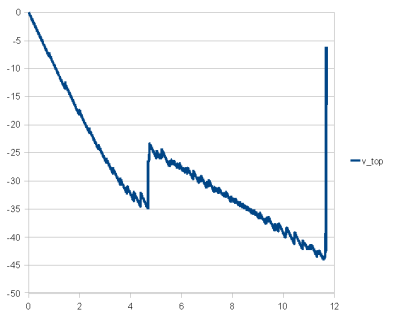
Can't miss that one.
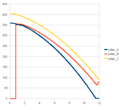
The next graph follows the displacement over time of the top of each zone. Zone B, of course, doesn't exist until the first contact and breakage, so is defined as having zero position until it exists.
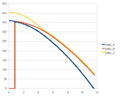
Notice how the complex curve of the top motion has been resolved into two distinct curves, the yellow and red. The crush up of Zone C, as well as its termination, seem to have little influence on the position of the other zone interfaces. Almost as if it could be treated as an independent problem. The difference between the blue and red curves depict the growing size of the crush layer, Zone B.
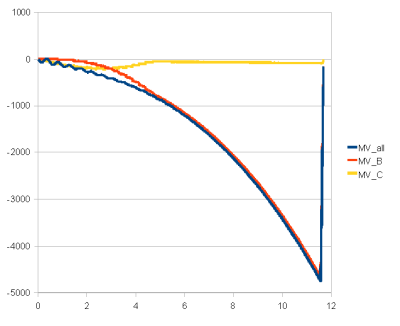
Less interesting, but still useful, is a graph showing the momentum possessed by Zones B and C as well as the total momentum (which includes 'stationary' Zone A, which can and does oscillate):
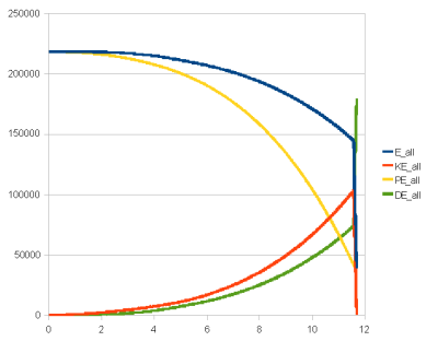
The distribution of energy over time shows the conversion from PE to KE with attendant losses from inelastic collisions and connection breakage. The green line is the accumulated dissipated energy:
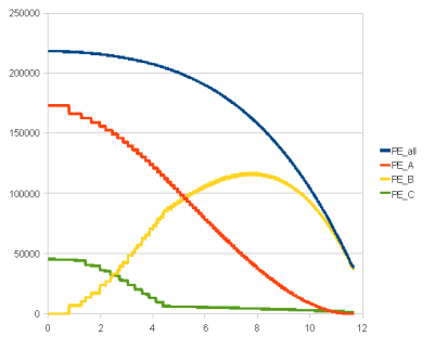
Potential energy distribution amongst the zones, against the total available, mostly reflects the changing distribution of mass of each zone, with everything going towards B and a gradually reducing amount because of descent:
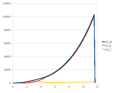
Kinetic energy, once crush up is done, is all Zone C for similar reasons:
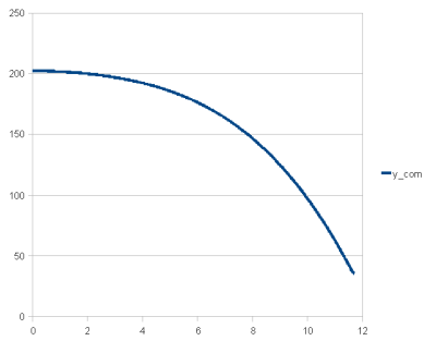
Turning back to displacement, this is the displacement of the overall center of mass, which is quite smooth:
Next will be the same model tweaked ever so slightly to promote nearly exclusive crush down in the beginning.
CASE 2- MOSTLY CRUSH DOWN
In these models, the upper block connections have uniform strength greater than the top connection of lower block. If the upper block is strengthened by a small amount beyond that of the previous run, it fares better, staying mostly intact until the bottom. The end of crush down in that circumstance is where the crude simulation departs from anything a real structure might do - Zone B, the crush layer, compresses then rebounds up to meet the falling upper block. A 400+m lattice of highly inelastic balls stops acting like a building at this point; it's fair to ask whether such a simulation acts like a building at any point. If not, can the same question be asked of any similar discrete 1D model?
Incidentally, it seems the only way to tame this crazy explosion at the end (can you say pyroclastic clouds?) is to artificially weld the slabs together as they become part of Zone B, then fix B to the ground when it hits. I can only imagine it would play havoc with the solver, and I don't see a big advantage over studying crush up separately when riding a solid block down at a fraction of g, something that will be well-behaved. But I'll try welding, too, probably.
The end of the curves, as a result, should be taken with the appropriate grain of salt. The initial crush mix looks like this:

while the bounce-up at the end is:

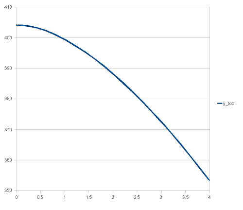
Displacement of the very top is a single smooth curve, instead of being two descents superposed.
Detangling the displacements by zone shows a different picture than the previous example. The reflection in the Zone B (red) curve at the end is the bounce up.
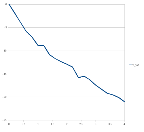
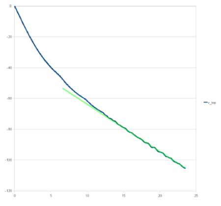
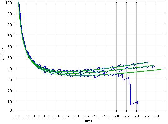
The speed of the top, which is the roofline, shows a series of relatively small jolts; small considering Zone A+B is a group of semi-rigid slabs falling together. The most notable features are the bend in the beginning and the linearity of the two segments associated with the fall.
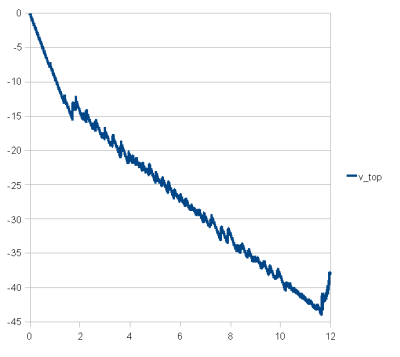
The first segment is essentially freefall, an unavoidable consequence of a simple slab model, the second segment is a shallower jaggy line composed of freefall descent peppered with jolts. Without high-resolution data, the line would appear straight with gaussian noise rather than unambiguously showing the customary sawtooth pattern of freefall punctated with jolts, as seen in this close up of the speed between seconds 4 and 6:
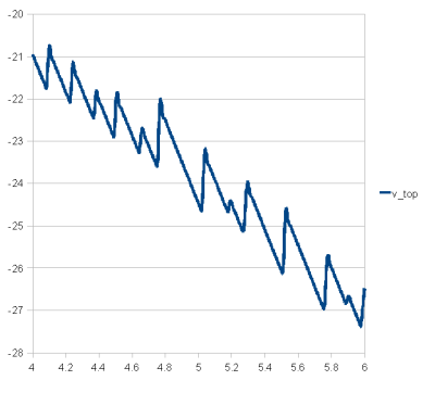
It's worth noting that this simulator gives an irregular pattern of jolts, simply because things are jostling around - as they would in the real world! The degree of similarity or difference between this and reality is one thing, the other things are the relationship between this and other models, their relationship to reality, and between different real scenarios. Is it more realistic to have uniformly regular collisions, as might happen in an analytical treatment which defines them to be so?
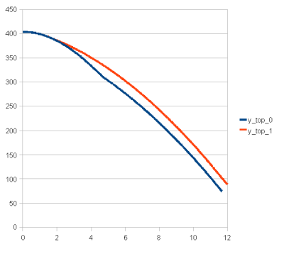
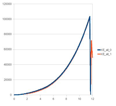
Comparing this example with the last reveals the gross differences in roofline motion but relatively minor differences in other parameters. The two collapses are virtually indistinguishable in the other measurable values. The previous example is labeled with suffix 0, this one with 1.
Displacement of the top:
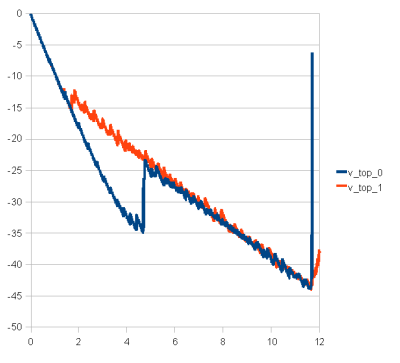
Velocity of the top:
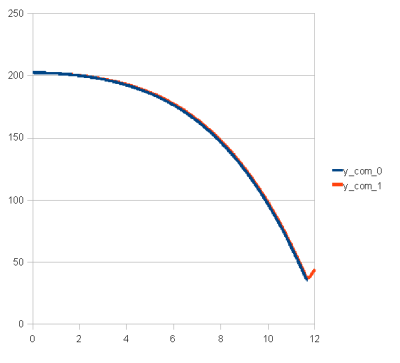
Displacement of center of mass:
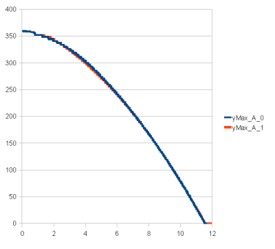
Location of top of lower block (crush front):
Total kinetic energy:
SOME OBSERVATIONS ON CASES 1 AND 2
If this style of simulation offers anything of value by way of comparison to physical progressive collapse, at least in these two examples, it is:
1) mixed crush direction should be distinguishable from exclusive crush down via roofline measurements of sufficient duration, by virtue of a faster descent
2) having mixed crush direction does little to alter the energetics of the overall problem, so ignoring it is OK (sometimes)
These observations run somewhat counter to my early intuition about the problem. I'd imagined simultaneous crush-up consumed more energy per unit time and would therefore leave less energy for motion. Wrong. The two 'reactions' occuring simultaneously liberate more PE per unit time by having the top drop correspondingly faster, roughly the sum of displacement due to crush down and up. Exactly so if defined as two decoupled processes, which seems a reasonable approximation.
Are these observations applicable to the real world? Is the real world WTC1, a 1D lattice of spheres - or both?
I think the lesson of top displacement under mixed crush applies generally to 1D models. At its core, the problem is approximately a loosely coupled pair of systems. The assumption of the prevailing theory, which is a continuum model, is that the upper block remains relatively undamaged until the end. I've read the part of B&L that addresses this (many times) and, while I understand the majority, I'm not in a position to check the validity of the work. I'll assume it to be correct and conclude that this is a significant difference with a discrete floor model - the upper block crushes up because it would if dropped onto a moving platform accelerating downward at a significant fraction of g, whereas in the case of continuous media this is not the case.
In a solid slab / stiff spring model like this, the initial collision is between two slabs which are coupled to other masses, NOT a collision between a rigid upper block and a single lower slab. The physics engine correctly applies the conservation of momentum to the two (mostly inelastic) bodies in contact. Then, based on resulting velocities of the bodies and forces transmitted through remaining connections, calculates the trajectories of the various pieces as independent bodies joined by stiff connections.
An upper block with the inertia of many members is not going to slow down much before the bottommost connection breaks and the resistance from Zone B is gone again for a time. Since the first collision is between two slabs, they move downward post-collision with half the speed of the upper block. The upper block catches up, breaking the lowest connection of Zone C, simple as that. The top will crush up right away unless the entire stucture is relatively weak and connection strength does not vary much going up. The other option is to make the top overly strong, as done here.
I wonder why the case of continuous media, discussed in B&L, differs so dramatically? Can an upper block that has experienced 10x maximum elastic deformation of its lowest story stand on its own at one-third gravity? Seems reasonable. How about when it's going to get smacked one more time before the ride smoothes out? Is not the extended treatment of B&L just a move of axiomatic rigidity one more story up?
One other thing falls out of this. Having the upper block be rigid as axiomatic does not greatly change the overall dynamics of a complete collapse, so seems justified from that standpoint. On the other hand, with such a simplified model that yet provides 110 degrees of freedom, violating this axiom (which is more realistic) sometimes leads to arrest.
ON JOLTS
About jolts. I just ran a 1D slab model, 110 story with 12 in the upper block. The upper block was made artificially stiff to force crush down first, with the connections set to the strength of the top lower connection plus a margin. The connections were such that the lowest could support 4x the imposed static load. The strength then scaled linearly up to the separation point, not terribly strong as you go up - it could go many times stronger towards the top before causing arrest.
Anyway, that's a little background. There isn't a stiffer situation to model, really, the upper block is a set of rigid masses coupled by very stiff springs. These springs break under minimal deflection. If there's going to be a jolt, it will be visible in this sort of system of discrete, axial strikes, where the only interaction is rigid body collisions, one per story. And they are visible.
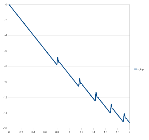
This is the velocity of the 'roofline' over the first two seconds of the simulation, 500 samples per second
Really obvious. Now how about the exact same data at 5 samples per second, first four seconds:
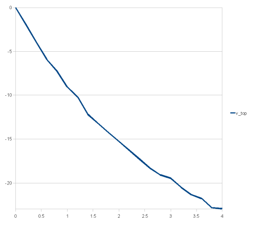
Not even a couple of flat spots, completely monotonic. Bearing in mind there's no video measurement error associated, this is about as much jolt as I'd expect to see when it is present, at that sample rate.
Not trying to pick on anyone, this is just something I've run across a lot and wanted to illlustrate. It doesn't matter if this is an accurate sim or whatever. It matters that the jolts are visible at one sample rate and not the other, exact same data.
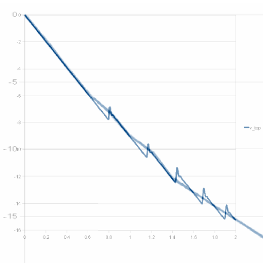
If it wasn't obvious, an overlay shows what's going on:
Another run with a stronger structure produced a flat spot and a jolt, even at 5 samples per second:
But... that's with perfect recording accuracy. Let's be fair. Here's the displacement curve that goes with the velocity graph, only at 500 samples per second:
The task is to digitize the curve using whatever method, whatever resolution you like. It's got to be easier than digitizing an edge frame by frame in a grainy video, it's a graph after all. Then take differences to get the velocity. Trust me, there are beaucoup jolts in this curve. We can compare results to the 500 Hz data coming straight out of the engine and see how well you did.
Then do the same thing with a generated graph of a parabola, just to see how jittery a straight line can be.
NEW CASES
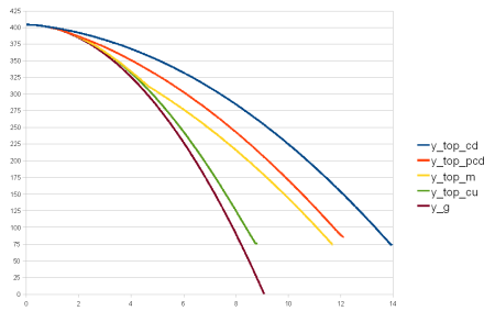
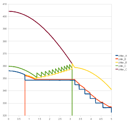
This is a comparison between various mixes of crush up and down in a 110 story structure. There are differences needed to get the desired results but otherwise similar structure strengths. Two of the cases are from earlier.
- the predominant crush down by artificially stiff top, the one with rebound (red)
- the more natural mixed initial crush down/up, two curves superposed (yellow)
New cases are:
- exclusive crush down using only the top (two?) floor(s) (blue)
- exclusive crush up by dropping ENTIRE building at lowest floor (green)
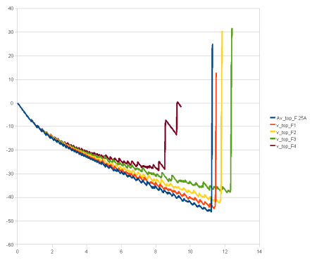
Finally, freefall is plotted in dark red for comparison.
All displacement
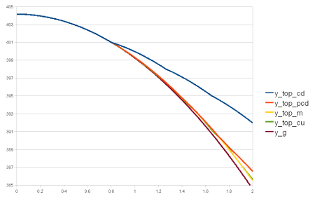
Displacement 0-2sec
All speed
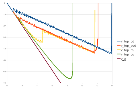
Comments:
Exclusive crush up is the closest to g. WTC7-ish. Without accurate hi-res measurements, there's little chance of distinguishing from freefall in the first 1.5 seconds. Exclusive crush down distinguishes itself early by 'skipping' like a stone on a pond, not a lot of mass driving from above and momentum transfer is a very big thing early on.
The velocity graph is more interesting. The yellow (mixed crush) matches the green (all crush up) until the upper block is getting small, then it starts to slow in a tail-off. When there's nothing left to crush up, it transitions abruptly over to the speed of the predominant crush down, which still has a mostly intact upper block. These two have the same acceleration as the exclusive crush down after four seconds, which is roughly constant (ignoring the bumps).
Constant acceleration of 0.3g, mostly
The constant average acceleration of the crush down portions is 30% of g.

([1 - stretch]*height/g = 0.3).
Compare to Energy Transfer, Stage 1
Time for a sanity check. Go back to the fundamentals, Greening's ET. Page 4, Stage 1 collapse time for WTC 1, 14 story upper block => 11.6 seconds.
If I make the joints of the lower block quite weak, but still well above non-existent, and the upper joints really strong to ensure crush down, I get a time of about 10.7 seconds - with a stretch of 0.2. With a stretch of 0.02, it's about 11.7 seconds. After a slight vertical offset to account for our different starting heights, it lays right on top of Dr. Greening's WTC1 curve.
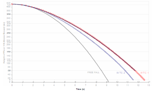
I think that passes sanity check. Not bad for 1kg floors, eh?
Varying stretch and connection strength
Might be useful to compare velocity of the last two runs, where the only difference was stretch. All the runs so far, unless otherwise noted, are 0.2 but, to match Greening's momentum only Stage 1 time, I had to go for high compaction.
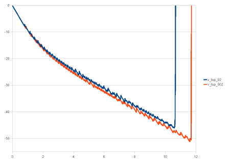
As noted towards the beginning of the thread, the biggest influence of stretch is make the fall longer or shorter. There is some difference in velocity, the higher stretch being a little slower, but the accelerations end up the same, and constant.
The simulator is not junk. It's a little difficult to reconcile a figure of 0.6g with 0.3g, however. Maybe WTC1 starts at 0.6g and goes to 0g, whereas this starts at g and goes to 0.3g, and it all comes out in the wash. ???
In another thread, there's discussion about how much momentum transfer counts, as opposed to resistance from structural strength. Dr. G made a comment about the falling rain drop problem, in reference to the similarity in mass accretion. He states:
Frank Greening wrote: ":The simple momentum transfer solution yields the result that the raindrop should fall at 1/3g, which is not observed for WTC 1."
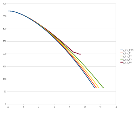
Time to investigate the effect of connection strength. ET says 2x overestimate of E1 adds only a half second to collapse time.
These runs use a single top slab with 10x the normal mass to crush down 100 floors with connection strength varying vertically at a ratio of 50:1 going up. The overall strength was set with multipliers of 0.25, 1, 2, 3 and 4x. At 4x, crush down arrested partway through. Not much more than a second's difference amongst those that go to completion.
Displacement:
Velocity:
Finally evidence of a different terminal slope!
Dissipated energy:
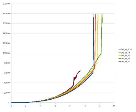
There isn't much difference in magnitude between the vastly different connection strengths, all of which are capable of supporting the structure. Compare the green and blue curves, which represent the difference in energy thrown to the aethers given by a 12 fold increase in connection strength. Most of the energy loss is from inelastic collision.
The arrest is interesting. A slight departure from the tight pattern becomes evident just before a huge step change as the lower block top slab is able to withstand one of the impulses from the Zone A/B mass. The gradient of connection strength is quite steep, though not quite as steep as the load gradient.
Energy dissipation and terminal acceleration
Typical cumulative totals of dissipated energy versus connection break count:
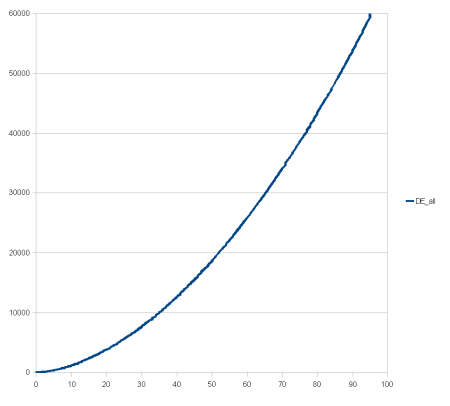
Nice blend of a parabola (velocity dependence in inelastic collision) and a straight line (connection count and strength).
These next comparisons are between 1, 10 and 100 mass units for the top slab crushing down 100 floors below.
Displacement:
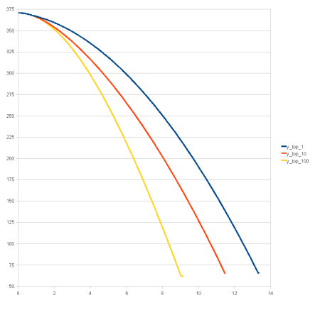
velocity:

Even with the 100x top mass, which is equal to the combined mass of all slabs below it, the tendency towards a similar terminal acceleration is suggested. Momentum transfer from collisions results in terminal acceleration as opposed to terminal velocity.
If the lower block were taller (200 floors) rather than 100, would the yellow velocity graph will level off to some near constant "terminal acceleration" like the blue and red examples?
It could be that it struck ground before it could reveal the slope at which it would level off.
I think so. Let's find out.
One 100x mass slab crushing down five hundred 1x mass slabs:
Just to clear up any possible confusion in what I said earlier, if WTC1 Zone C is riding the elevator at two-thirds g, it's like being in a one-third g world. Coincidentally the sims come in at g/3 which is like being in a two-thirds g world. Will the virtual structure crush up at one-third g? Yes, it will. Even at one-tenth g.
Comparison of displacement over time, g and g/3 fields:
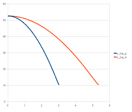
Not entirely fair to compare with simultaneous crush down, because the initial average acceleration there is close to g, the impacting slabs start with an initial velocity of half the upper block and freefall down to the next slab, as does the upper block. Not the same as a crush up into ground at one third gravity, but still useful.
another validation of the engine:
In Bazant and Le: "The acceleration (v_B dot) rapidly decreases because of mass accretion of zone B and becomes much smaller than g, converging to g/3 near the end of crush down (Bažant et al. 2007)."
About the wavy velocity line. 500 stories is about the limit. Not for the physics engine, but for the structure. 1850m tall, 0.74m wide, amazing that it stands at all. Maybe it wouldn't, haven't tried the static structure over time, but at least it doesn't break anywhere but the crushing front. There's so much flexure, the lower block has quite a few waves traveling back and forth during collapse. Sort of a Tacoma Narrows bridge thing going on, it can be seen in the bumps of the velocity curve. Those aren't jolts, they're resonance effects. Repeated slamming at the peak strength of the connections.
In this sense there's no cheating with the engine. Want a rigid block? Better make it that way or it might crush up. Think all the energy is dissipated at the crushing front in a 500 slab structure? Nope, it isn't. It's not how real-world materials behave, it's not how virtual world materials behave, either. Choose E1 carefully. The structure has to stand under its own weight; too strong and it refuses to break.
The other side of the coin is pushing the engine into bad behavior, something I've managed to avoid lately, but it was not without a good deal of time spent in trial and error. Even things like choice of time slice (with the consequent binary floating point representation, not so much the size) have a profound influence on the stability and accuracy. Now, having found the sweet spot, and having a good idea of the warning signs when things go awry, I'm pretty confident of the 1D results so far. Moving to more elaborate models, and then 3D, will bring new considerations and perils. My hope is to be able to get good simulations of matter transitioning from lattice structure to granular, near-fluid state under the influence of internal defect and its own weight, spanning a variety of conditions and configurations.
The 1D behavior is most curious but fortunate. Without it, there would be little hope of recreating these 'ideal' 1D analytical scenarios using this system. Turns out spheres in a vertical line will stay on the line, even bouncing at high speed elastically. Real slabs go 3D immediately, with rotation and asymmetry, but spheres are stably 1D in this arrangement. Actually did some 1D gases, helped to work out the kinks in the system.
Comparing largely inelastic to largely elastic collisions
In the engine, this is mostly governed by the restitution property of the colliding bodies. For inelastic, this value is set to zero, which does not provide the textbook definition of fully inelastic because of the object skin mentioned earlier. The elastic trial uses a restitution of 0.9 for both bodies, and there's quite a difference between that and 1.0, the maximum.
Perhaps surprisingly, there's not a tremendous difference between the two extremes. Slabs that can rebound more get involved in more collisions, which dissipate energy quickly. For this reason, I include a graph of collision count per timestep (which is small at 0.002s). The net effect is little difference in other quantities for such a drastic change in material properties. The crush front does not race wildly ahead of the inelastic case.
Top displacement:
Kinetic energy:

Dissipated energy (tail included to show there IS a difference at the end):
Crush front location:
Collisions per timestep:
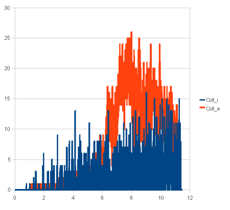
Note the elastic case reached a maximum collision frequency of around 12,500 Hz! Normally, that wouldn't inspire much confidence in the simulation but it actually behaved quite well by every other standard. Outwardly, it was barely distinguishable from inelastic, which has some pretty high transient counts as well. Plenty of collisions for recrushing, or a smaller number of more energy-dissipating collisions, doesn't seem to matter much in observables.
On Stretch
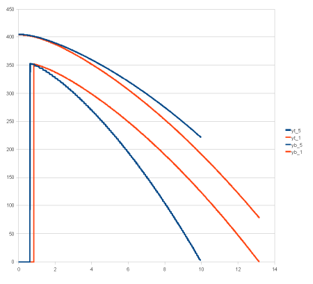
The subject of stretch came up in the other thread, so I thought I would delve into it a little more. It's the reciprocal of the compaction ratio, which may be more intuitive but is sometimes less convenient. Here is a comparison of two extremes, 0.1 and 0.5. The latter has the 'special' property that, upon collapse completion, the pile is half the height of the original structure. Obviously, this has no relation to anything significant, it's just to illustrate how stretch affects the measurables in what is an accretion problem.
These are the roofline and crush front locations, red is s=0.1 and blue is s=0.5:
This graphic overlay depicts the region extents at start, mid and end:
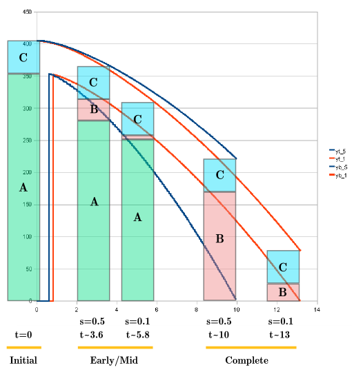
The obvious conclusion is that increasing stretch results in higher/slower roofline displacement, and relatively greater magnitude change of crush front displacement in the downward direction. Later, I'd like to explore some curve fits and interpolations, but this lets me close those spreadsheets.
Delayed crush-down
Oh yes, one other oddity. Initial drop breaks one lower connection, then there's a sustained, exclusive crush-up followed later by re-initiation of concurrent crush down. Unfortunately, I don't remember much about the conditions, and I don't want to look them up in the archived index. Undoubtedly, it was contrived. Locations of Zone A/B/C limits over the first five seconds:
On 1 Dimensional Modelling
At this stage, it may be worth mentioning that the 1D world really hasn't outlived its usefulness. There is more accumulated info on simple 1D simulations than what's been posted here. The applicability is not immediately obvious, so going through ALL of the details to show the limited usefulness is questionable. The most interesting was attempts at systems akin to 1D gases. Originally, the purpose was to get a handle on the behavior of the simulation engine with as few variables as possible. I'd already done very simple 3D systems with quite chaotic results and it seemed appropriate to limit the system even more to ensure this was not just a stupid cartoon generator.
Fortunately, I found that spheres in original 'perfect' alignment stay in alignment so long as no lateral forces are introduced. I find this remarkable, and interpret it positively in regards to the stability of the engine. While no set of real spheres would exhibit this behavior, in theory the divergence is easily explained by the sensitivity of the problem to minor variations in placement, surface irregularities, deformations, and so on. In experiment, the same set of balls dropped with the best precision possible would display radically different trajectories and final positions because of these factors. Only statistical generalizations about the system can be made and results from simulations can contribute to this picture if run in large numbers with small (semi) random variations. The point is, without sufficient descriptive knowledge to build into the simulation, any particular run is of limited value in a chaotic system.
Consider how that may apply to the NIST simulation. While indeed 'detailed', it can easily be argued that it is not detailed enough to ensure convergence on the proper specific solution if one is sought, and that it is too detailed to represent insensitive, gross characteristics.
The spheres in PhysX behave well in the sense that no lateral force component is spuriously introduced via approximation tricks, floating point error and what have you. What is a 3D simulation then acts as if it is 1D. With that, multi-body collisions act in a (more) tractable domain so it's easier to set up systems that have grossly predictable behavior and see how well the engine does. In the course of doing so, several non-physical glitches became apparent, mostly in the area of time increment, and strategies to avoid bad behavior could be formulated and verified.
In the 1D gases, there is an opportunity to explore what happens when there are many collisions occuring between a multitude of bodies, in terms of just a few simple scalar parameters and numeric results. A 1D gas, in this context, consists of free bodies moving on a vertical line under the influence of gravity. The entities cannot cross paths, so maintain the same ordering. In one set of experiments, the top sphere was made much more massive than the collection below, so functioned as a (piston-like) load applied to the gas. The 'temperature' of the 'gas', as in statistical physics, is based on the ensemble kinetic energy. Initial temperature is set by assigning random initial velocities in the one dimension, then the system evolves under the influence of gravity and the applied load at the top.
Naturally, the system will bounce the load. If the restitution property is large enough, it can bounce indefinitely. In any case, the system behaves as a harmonic oscillator with a characteristic period. Since many real-world building materials have a non-trivial coefficient of restitution or, more appropriately, do not exhibit fully inelastic response to collision, the 1D gases helped characterize what can be expected of the simulator when restitution is varied. Previously apparent was, in general, the more chaotic simulations resulted from introducing elastic behavior in the members. While this may or may not be more realistic in any given sense, to get useful results while avoiding the need to do thousands of runs with minor variations (discarding the obvious failures), restitution must be set to zero and sometimes additional damping introduced to keep things from blowing up. Unfortunate, but true.
Where the gas study helped was in observing that the engine was capable of simulating pressure, that being the result of internal kinetic energy of an isolated portion of the system transferring momentum to another portion via high frequency (essentially discrete) collisions. Pressure from rigid body mechanics.
In one collapse sim earlier, I let the collisions be mostly elastic and it didn't change things much. I'm not sure what femr2 did in the async sim, but it looks like it went a little nuts. If I let the restitution be unity, my sims go ape, too. Clearly this is not a fruitful avenue; intuitively, there's no reason to expect the failure to propagate upwards in a 'fracture wave' (at least in this manner) and certainly there isn't much in the way of evidence to support it.
However, that's not to say that damage cannot propagate well away from the average location of the crush front, due to preservation of KE post-collision in the internal degrees of freedom. But, when you consider issues such as mean free path and average time between collisions, it's not obvious to what extent that can occur in real life. Higher restitution means higher post-collision velocity, which in turn means more frequent collisions. Thus the KE still gets drained off rapidly for reasonable values of restitution, a non-linear effect in a confined system.
Later I may post some of the 1D results of non-collapse systems, but I think this covers the gist of it. Where there is still some ground to explore in 1D is in composing 'stories' from spheres of non-uniform properties, as opposed to having a single sphere to represent a concentrated, rigid slab (which paradoxically is also inelastic). I believe that a very crude approximation to story density, compressibility, and elasticity can be incorporated which would make the sim more realistic than slabs. A story unit can then have internal degrees of freedom and exert pressure on its surroundings. Work is done against a virtual resistive force applied over distance instead of discretely once per story, stemming from repeated collisions and more gradual entrainment of mass.
Varying cap mass and connection strength
This experiment is to determine the influence of cap mass, similar to ones done previously but with a pair of tests using different connection strength schemes to determine the influence there as well. The configuration is 100 stories, upper block consists only of topmost slab which drops onto the remaining structure and crushes to completion. Except for the top slab, slab masses are identical; the top slab mass is varied through 1x, 2x, 4x and 8x the normal slab masses as a varying parameter. The slabs are 0.2 x story height, AKA 0.2 stretch or 5x compaction.
These are also at least minimally self-supporting structures, they would continue to stand if not for the split introduced as an initial defect. This is necessary to conduct the experiment by definition, but it imposes certain constraints on the construction scheme. As the top mass is increased, the structural capacity in terms of joint strength must also be increased, so mass is not the only variable in the simulation, energy lost to joint breakage is also variable.
Many previous experiments used a simple scheme where the load at each level determines the joint breakage force to within a scaling constant. This results in the lowest connection of a 100-story structure of uniform slab mass being 100 times stronger (in terms of peak impulse, at least) than the top connection. That's not too realistic in the context of skyscrapers, but that does bring up an interesting point: when someone says (e.g.) DCR of 0.5, that can't apply throughout the vertical extent or you do get a situation where the ground story is 100x stronger than the top.
To illustrate the influence of connection strength gradient, a pair of trial sets are done with:
- a linear gradient of 100% capacity required at the bottom to 10% of that value at the top
- a constant connection strength all the way up, set to 100% capacity required at bottom
The latter has the necessary bottom connection strength all the way up the structure, but overall capacity was reduced to the minimum reasonable amount to ensure crush down could occur even at lowest slab mass, one-third the capacity of the first set. Thus the energy consumed by connection breakage, while not presumed to be identical, may be similar in both sets. It is the difference in capacity gradient that will be explored.
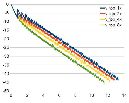
Raw displacement and velocity -both cases
The linear gradient case for 1x/2x/4x/8x top slab mass.
Displacement:
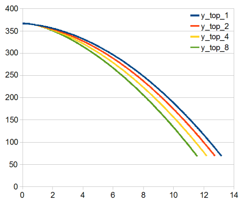
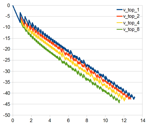
Velocity:
====================================================
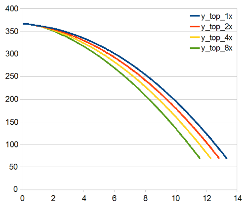
The flat (no gradient) case for 1x/2x/4x/8x top slab mass.
Displacement:
Velocity:
Interpolating the velocities
If you compare to the graphs posted in the referenced War Wheel thread, the immediate obvious difference is that this scheme does not result in the final velocities ending up the same in each case, the heavier ones are faster - all falling the same distance. Otherwise, there's not much discernable difference amongst any of the different schemes, shape-wise.
Because the data coming from the physics engine is not a measurement, rather the result of a calculation, it isn't subject to error or noise. The jitter in the velocity trace is the series of jolts from collision, with the snap-back characteristic of the many-jointed chain. This velocity data is perfectly good to use for the purpose of obtaining a good analytical interpolation and then differentiating to get an approximate acceleration curve.
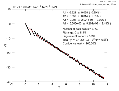
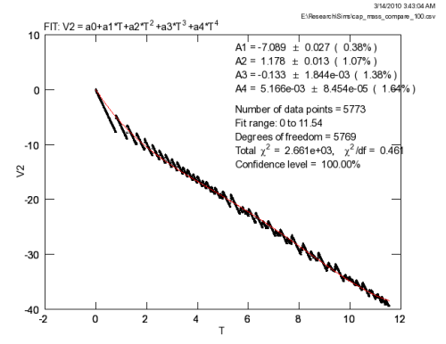
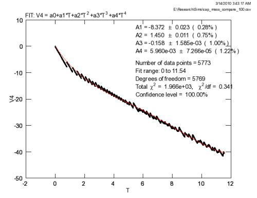
I chose a 4th degree polynomial for the fit, for no special reasons other than I thought 3rd degree could provide a good fit to varying acceleration after differentiation. The constant (offset) coefficient was set to zero as a boundary condition. The latter end (not fixed) of the sets is not quite such a good fit as the front, so I would de-emphasize the particulars of the trailing end of the interpolations and especially derivatives. Sets have been trimmed to a common length of time.
I show this work for the linear gradient case:
V1: velocity for cap mass of 1x
V2: velocity for cap mass of 2x
V4: velocity for cap mass of 4x
V8: velocity for cap mass of 8x
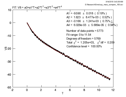
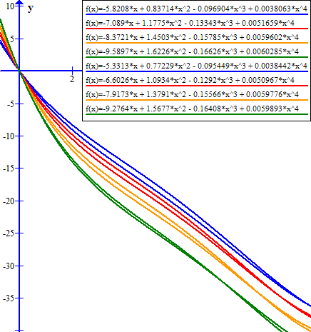
and present the equations for both cases:
********************* FIT RESULTS **********************
Linear 100% - 10%
********************************************************
V1 = -5.8208*x + 0.83714*x^2 - 0.096904*x^3 + 0.0038063*x^4
V2 = -7.089*x + 1.1775*x^2 - 0.13343*x^3 + 0.0051659*x^4
V4 = -8.3721*x + 1.4503*x^2 - 0.15785*x^3 + 0.0059602*x^4
V8 = -9.5897*x + 1.6226*x^2 - 0.16626*x^3 + 0.0060285*x^4
********************* FIT RESULTS **********************
Flat 100%
********************************************************
V1 = -5.3313*x + 0.77229*x^2 - 0.095449*x^3 + 0.0038442*x^4
V2 = -6.6026*x + 1.0934*x^2 - 0.1292*x^3 + 0.0050967*x^4
V3 = -7.9173*x + 1.3791*x^2 - 0.15566*x^3 + 0.0059776*x^4
V4 = -9.2764*x + 1.5677*x^2 - 0.16408*x^3 + 0.0059893*x^4
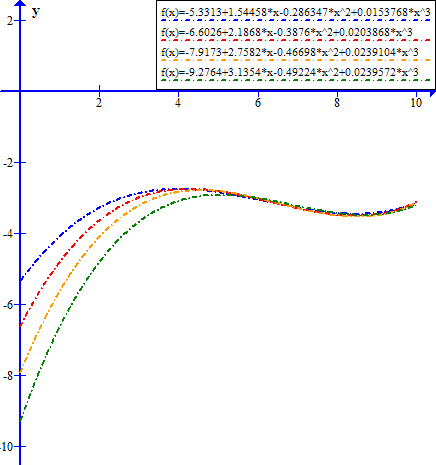
Velocity and acceleration from interpolation
The velocity fits for the linear gradient:
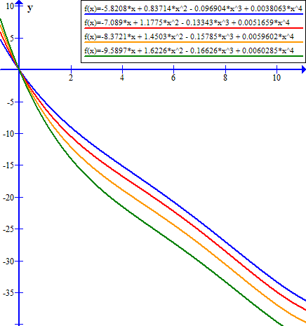
and the accelerations obtained by taking the derivative of the interpolation:
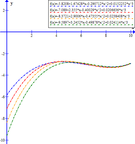
======================================
Velocity for flat:
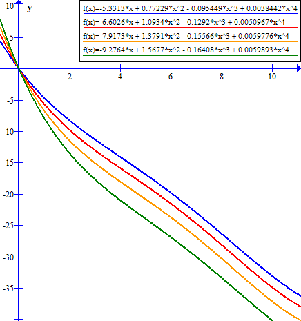
Acceleration for flat:
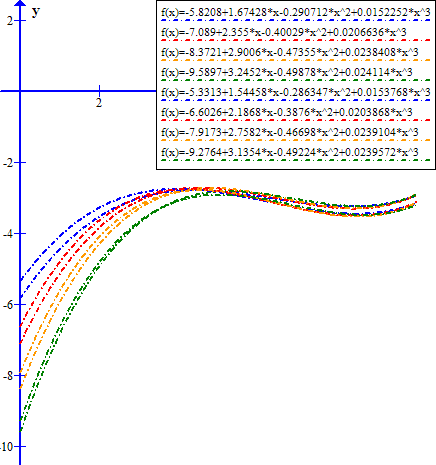
======================================
Both overlaid, velocity:
Acceleration:
The actual collapse times differ, from lightest to heaviest, by about 2 seconds. That's not insubstantial, but perhaps not as much intuitively expected when scaling up the mass 8 times. The overwhelming factor is having to plow through a line of masses that add up to much more than the original mass, even at 8x top load.
Once again, the rough convergence on a single constant acceleration value is seen - terminal acceleration. The interpolations indicate a sort of oscillation rather than asymptotic approach - but, again, I wouldn't read too much into it past 5 or 6 seconds in. Not to say there isn't something of interest there, but it will need to be studied further. Same with the crossover point of the clusters towards the end.
The linear gradient, as expected, exhibited slightly higher initial accelerations than the flat counterpart because the flat is stronger higher up, but both join by about three seconds in. Less than 5 seconds into progression, all trials have about the same acceleration, around one-third g. By this time, there is a fair difference in the velocities seen with the different masses, but this difference will remain fairly constant and represent a lesser percentage discrepancy against the overall average velocity the longer the collapse continues.
Didn't you show (on the other thread) that even a 50/50 split demonstrated this effect?
Almost. The reason 50/50 doesn't work out so well is there's not enough distance to fall with a split before a certain point. If you think about it, splitting at the first floor (bottom), even though there's 109 stories above as a driving mass, and it freefalls through one story, there's only one story to drop.
Did a series of runs on a 100 story structure with splits every tenth floor:
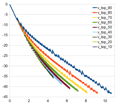
Comparing 1D models, high velocity initial impact
Been working on a step-wise crush calculator, here and there. The two processes can help validate each other. In working out some of the kinks with both the 1D physics engine simulation and the complementary stepwise algebraic version, a few interesting things popped up.
Most of the time there's a really good match between the two methods:
Overlays of positions
- physics simulation and stepwise computation
- varying top impactor velocity
Sometimes there is a significant divergence:
Comparison of velocities
- physics simulation and stepwise computation
- 1000 m/s impactor
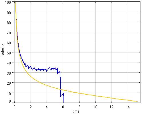
The jagged blue line headed south is the physics engine model arresting a 1000 m/s single slab impactor six seconds into crush. The arresting model had only an equivalent average resistive force of less than 0.25m(t)g from supports; the same in the stepwise computation begins accelerating again during this time. The difference is that the debris zone in the phyics simulation is free to wiggle about up and down, though the slabs are inelastic (zero restitution) they still slap about a little and approximate 'loose(r) debris' if only in a 1D sense. This is in contrast to the fusing which occurs by definition in the stepwise model - the debris zone as well as the upper block is rigid. This turns out to matter more in some cases than the rigidity of the upper block.
A number of things came out of this calibration exercise, aside from a few minor bug fixes and a maxwell line of 0.0237*mg*fos determined for the fixed joints in the simulator. The two images are the bookends of the exercise.
What is the point of investigating the results of 1000 m/s drop speeds? Curiosity and calibration. Based on more everyday (? by that I mean one day out of all of history versus never) conditions of the speed of a single story drop, I'd ascertained the values of a couple of parameters that are key in step-wise calculations, the average equivalent resistive force over a story and the effective compaction ratio. By showing these values to be consistent even into extreme conditions, the stability of the simulator is confirmed. Having reliable values allows direct comparison of trials using both methods with the same input, as was done for the graphs above.
The stepwise calculator is in work, but usable. There were small disagreements between it and the physics simulation, primarily stemming from ill-defined story counts in the zones. I was forced to think about this problem and resolve it in order to calibrate against the analytical model. For example, a crush down involving a rigid upper block of 1 story leaves the top story intact at the end. Since one story is as small as the upper block can be, it means a collapse can never be complete under this scheme if exclusively crushdown. The top story can crush up (but as Bazant notes, even this cannot fully complete the crushing of the story!) but an exclusive crushdown leaves a minimum of one story behind, an intellectually untidy affair to me but one that was never a concern until trying to relate results to the slab model in the physics engine. Since the physics sim starts with slabs already 'compressed' and just lets them collide, a single story upper block is already compacted and the final pile height from the y_top coordinate is different.
This is, at its computational heart, less of a philosophical issue than an off-by-one index thing, but I decided to address it in a philosophical way by making it so the top story could crush itself and an exclusive crushdown could then go to completion as an exclusive crushup can, a thing of wonderful symmetry. Physically, one can think of it as having all the story mass concentrated in the compacted slab which is now top-justified within the story height, instead of bottom-justified as I'd done earlier, and which is perhaps more intuitive but not necessarily more realistic: the slab and office contents for the bottom story is at ground level and gets crushed but does not drop; the topmost slab is really the roof. Of course, this is what happens when trying to pigeonhole non-uniform structure into a uniform model. Both models allow each story unit to be configured in any desired way, but most basic experimentation is done with as much regularity as possible to keep it simple and explore the basic parameter space completely before moving on to greater complexity in structure.
The floor indexing strategy is just a bookkeeping thing to get the position-time values to match between the models and allow the roofline to reach ground level in the case of infinite compaction. None of the mechanics has changed. The strategy is not necessarily optimum or even finalized, but it will do for the time being.
It is quite satisfying to see two radically different means for computing solutions agree so precisely. The processes are not the same, though, so they should not be identical under all conditions, and they are not as the second graph above indicates. Exploration of the differences and reasoning about causes should be a fruitful avenue. Along the way to obtaining calibrated sim parameters, the difference between the two processes became evident under certain conditions where loose debris slabs and elastic structure differed significantly from rigid bodies (in ways quite intuitive). I'll post some of the highlights next.
In summary, in a 1D full entrainment model, the dynamics of collapse do not differ much between strictly rigid zones versus slab-spring/loose slab, but the dynamics of arrest can be radically different.
Caution is always advised in generalizing from the very limited conclusion drawn, however this is is solidly on track with the observation that a sack of flour will do more damage if dropped on your head as opposed to poured out. It starts to put numbers to the notion, though with the crude granularity of only a few mono-sized particles. The most severe limitation is the 1D aspect, with the particles constrained to interact along a line with only their nearest neighbors. I'm afraid the rules will change drastically with the addition of spatial dimensions, and the possibility of flipping (many times) on this general principle based on conditions will be high.
If collapse goes to completion in a momentum-only (no supports) inelastic configuration, then the entire event can be considered a single inelastic collision in the sense that the final velocity of the debris pile just before hitting ground is that given by a collision between the upper block and the lower block as point masses - ignoring gravitational effects, of course. So, in a horizontal arrangement of inelastic slabs, a single impactor hitting a line of 99 masses has the collective debris zone speed reduced to 1/100th that at the final collision. Makes perfect sense.
It also provides another means of validation of calibration obtained under other conditions. Here, the initial downward speed can jacked up to ridiculous amounts, so long as the time step is made sufficiently small. I chose a single top slab v0 of 1000 m/s to slam into 99 floors below under a variety of circumstances. In the stepwise model, it's only necessary to set support energy to zero to run with momentum-only, but the physics sim is like real life in that a stucture with no supports will fall uniformly at g. It would be possible to make the supports disappear at the right moment but it's more effort than I care to expend on it. The solution to get momentum-only is to turn gravity off. This is one of the cases presented next.
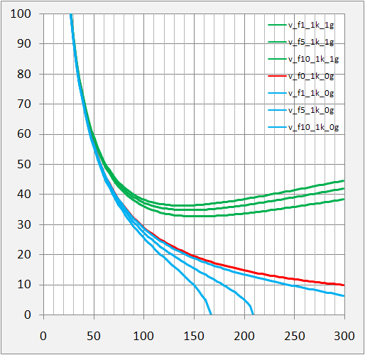
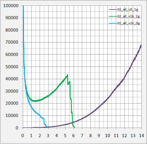
The graph below is a plot of top slab velocity vs time for 7 different impact scenarios all at 1000 m/s (plus delta for drop height of 0.8*3.7m in gravity cases). The green lines are with support in 1 g field, the red line is no support in zero g, and the blue are with support in zero g. Three support capacities corresponding to FOS of 1,5 and 10 were used in zero and 1g. The stretch and maxwell numbers are 0.196 and 0.0237 (@ FOS = 1).
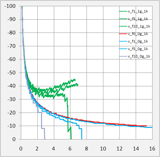
Of the seven cases, the momentum only red line cannot arrest because it's the only one which has no support. This exemplifies the kind of collision transaction alluded to above. By completion, it's equivalent to a single inelastic collision between two bodies of masses m and 99m. When support fail energy is added, the results change in a regular way about the special trajectory of the red line except for arrest.
Three of the six remaining cases arrest, two under zero g and one in gravity. The one in gravity is the arrest case portrayed in the second graph of the earlier post. The similar case in the stepwise model does not arrest. What are the differences?
1) In the physics simulation, the slabs are connected by joints that are short travel non-linear springs. Several things remain in characterizing their dynamic behavior but this exercise has shown their energy consumption under failure to be consistent under a variety of settings. In high FOS trials, the bottom slabs are observed to recoil significantly with each impact above, indicating the joints absorb energy. They seem to be highly damped, like a shock absorber. This is an energy sink not accounted for in the stepwise crush calculator, but it could be in a generic way.
2) The slabs collide mostly inelastically in the physics simulation, but not perfectly so. There is a repulsive skin depth because singularities don't solve well in any system, and there is some elasticity. Because of this, the slabs in the debris zone will be loosely packed instead of artificially and unrealistic welded on collision. This results in a vertical newton's cradle sort of affair when impacts occur, and these repeated inelastic collisions dissipate energy.
Item 1 is not really characterized in any way other than the appearance of damping. The propagation of shock waves through this medium is undoubtedly peculiar to this bizarre structure of 1D semi rigid spheres and highly dissimilar to any real macroscopic system of interest.
Item 2 is quite a bit more realistic for physical slabs like tiles than the analytical model of accretion, however the analytical model may be more like real buildings than rigid slab approximations. To the extent that debris was loose, it applies but doesn't go far enough, it just hints at what the characteristics are in a discrete 1D model with relatively small numbers of particles.
The area under the velocity curves above are the total distances traveled, obviously. Those trials going to completion all have the same area.
The green lines, with gravitational attraction added as a driving force, are dramatically different in nature from the zero g (red and blue) in which initial kinetic energy of the impactor is the only energy input to the system. At only 0.5 seconds in, the velocity has decreased tremendously in all cases, but by 1 second the greens are already splitting off noticeably. By 2.5 - 3.0 seconds, the green lines have hit a minimum of velocity and are beginning to accelerate again!
This is the difference gravitational potential energy makes.
An average force at each story of 0.1185m(t)g (FOS=5) can arrest a unit mass impactor in just over 7 seconds but, with gravity, the same structure goes to completion in slightly less time. The oddball, though, is the FOS 10 case with gravity. It arrests in 6 seconds.
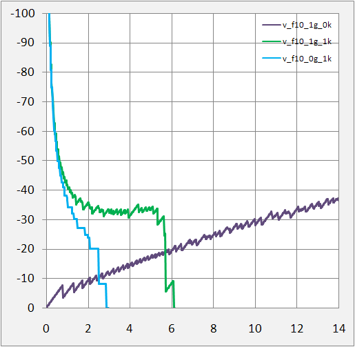
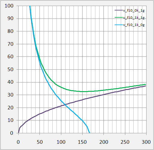
How do the two FOS 10 cases above, 1g and 0g, both of which arrest, compare to a single story drop of one slab on 99? The two cases above are shown below in the same color along with a third line which is a single slab drop initiation in a gravity-driven collapse. It goes to completion!
The previous three cases will be examined in greater detail shortly. In the meantime, here is a similar pair of graphs for the same configurations done in the stepwise calculator. The big difference is that these are in the spatial domain; that is, plots of velocity versus position instead of versus time, because the step increment is spatial in the stepwise calculation. Kind of an interesting twist. The two zero g cases of FOS 5 and 10 arrest as in the physics sim, but none of the 1g runs arrest.
To recap, there were a series of physics engine simulation where one slab was 'fired' downward at 1000 m/s, instead of simply dropped, onto 99 slabs below. As the support capacity was increased incrementally, the progression was arrested as shown in the graph above which compares against a pure analytical result of the same configuration which does not arrest:
The 1000 m/s impactor cases were compared to a simple top slab drop of one story with the same support capacity as the case which arrested.
The passive drop collapsed to completion! This is curious and demands an explanation. Is the engine screwing up? No. It is an artifact of the configuration but the engine is performing correctly. It turns out to be the two factors I mentioned above - lack of rigidity in the debris zone and the lower portion, interacting in subtle but important ways to reach a condition where the impulse train from above can be resisted by the lower portion and collapse arrested. Detail to follow.
Comparing against an analytical result which arrests in the same time, the stepwise model had to have support capacities increased 3.7x. This has been added to the previous graph of stepwise results showing velocity versus displacement (the orange line):
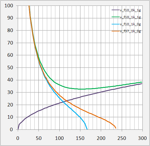
With this capacity, the curve much more closely resembles the blue curve at zero g, much lower capacity.
A comparison of the velocity for the original arrest and the new stepwise arrest at 3.7x capacity. The arrest is gradual in the stepwise case, as is the norm.
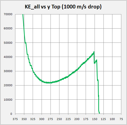
A look at the KE of the physics sims only shows that the arrest is abrupt (already knew that) and that it occurs at a much higher energy than the standard collapse and while the KE is in a phase of rapid increase. What's going on here?
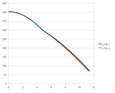
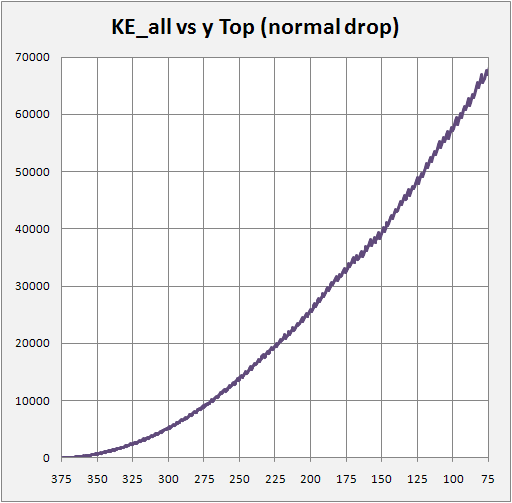
The previous graph compares KE in the time domain, but that's not an entirely fair comparison since the high speed collapse crushes much more structure per unit time. These two graphs compare the KE of the high speed and normal collapse against position. Still, not too revealing but this time we see the KE is actually comparable by the collapse position.
High speed:
Normal:
Note on the values/units - these are kg-m-s newtons, joules, etc, but I (typically) use unit masses because the dynamics are the same. However, this makes energy values very small, and of no use for comparison to other models which use skyscraper-like masses.
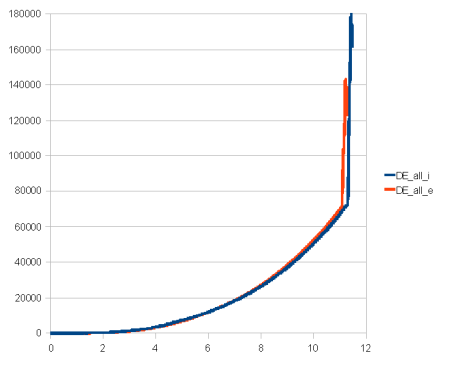
The amount of energy dissipated by the high speed cases dwarfs that of the normal collapse.
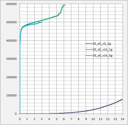
The rate at which the high speed cases throw energy away early on, without comminution or pulverization, is incredible! All momentum transfer, and it happens in the first few collisions. The configuration of rigid slabs is not realistic in this case because the inelasticity is by material property decree and not by virtue of something that could behave like that in real life.
Still it is amazing how quickly the dissipation slopes stabilize to something similar to a normal collapse. (although nearly constant for the high speed arrest)
Zooming in on the critical portion of time around arrest:
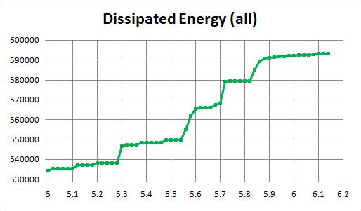
Suddenly there are big steps, where there were only smaller ones after the displacement stabilized. Where does this energy go?
Let's look at the momentum of the whole structure as well as the parts to see if there are any clues.
This is total momentum over the entire collapse period:

Zooming in on the arresting portion:
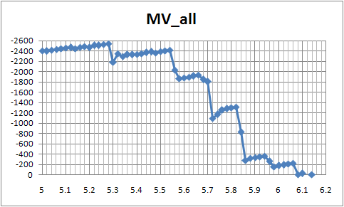
There is something interesting happening right after the downward steps, particularly just after 5.7s where something sort of slow and sustained is happening - momentum increases after an abrupt drop. There are signs of elastic rebound.
Turning to the momentum only for zone B (debris):
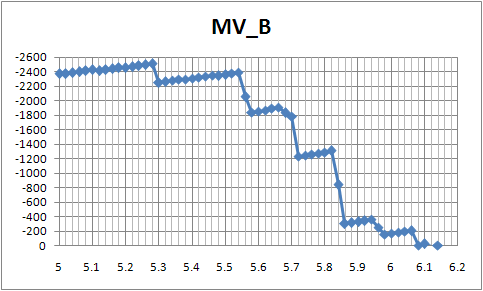
There's a bend downward at around 5.65 sec but a straight line starting just after 5.7. The debris zone is not responsible for the bend at that time.
Zone A, the 'fixed' lower portion:

The lower portion goes into motion
1 The study is extracted from a forum thread named Solid mechanics simulacra, of the toy variety, linked here.